1. Modeling & Simulation#

from estim8.models import FmuModel
from estim8.visualization import plot_simulation

1.1. Mathematical model formulation#

The workflow is demonstrated using a simple Ordinary Differential Equation (ODE) model from the field of biotechnology.

Here, growth of a microbial strain (biomass) in batch culture can be described in the form

(1)#\[\begin{equation} \frac{d}{dt} X(t) = \mu(t) \cdot X(t), \quad \quad X(t=0)=X_{0} \tag{1} \end{equation}\]

where the biomass is denoted as \(X(t)~[g~L^{-1}]\) with initial concentration \(X_{0}\), and the specific growth rate is denoted as \(\mu(t)~[h^{-1}]\).

By taking a black-box approach and assuming a single finite carbon and energy source denoted as \(S(t)~[g~L^{-1}]\), the growth rate can be modelled by a Monod-type kinetic in the form

(2)#\[\begin{equation} \mu(t) = \mu_{max} \cdot \frac{S(t)}{S(t)+K_S} \tag{2} \end{equation}\]

where \(\mu_{max}~[h^{-1}]\) denotes the strain and substrate specific maximum growth rate, and \(K_S~[g~L^{-1}]\) the half-maximum saturation constant.

The depletetion of \(S(t)\) in dependence of microbial growth can then be modelled as

(3)#\[\begin{equation} \frac{d}{dt} S(t) = \frac{-\mu(t) \cdot X(t)}{Y_{XS}}, \quad \quad S(t=0)=S_{0} \tag{3} \end{equation}\]

where \(Y_{XS}~[g_X~g_S^-1]\) denotes the biomass specific yield coefficient.

1.2. Model implementation#

The model is implemented using the modeling language Modelica as shown below. OpenModelica offers an open-source and interactive environment for this purpose.

model SimpleBatch

  // define real states
  Real X(start = X0, fixed = true);
  Real S(start = S0, fixed = true);
  Real mu;

  // define variables
  parameter Real X0 = 0.2;
  parameter Real S0 = 10;
  parameter Real mu_max = 0.4;
  parameter Real Ks = 0.01;
  parameter Real Y_XS = 0.35;

equation
  der(X) = mu*X;
  der(S) = -mu*X/Y_XS;
  mu = mu_max*S/(Ks + S);

// prevent negative substrate concentrations
 when (S<=0) then
  reinit(S, 0);
 end when;

end SimpleBatch;

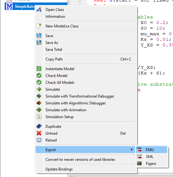
To apply this model with estim8, it has to be exported as a Functional Mockup Unit (FMU). Both FMI types Co-Simulation and Model-Exchange are supported. With OpenModelica, this can be done by right-clicking the model class and following the steps below.

1.3. Simulation with `estim8.FmuModel`#

The FmuModel class offers a Python-based simulation interface for FMUs. For initialization, simply pass the FMU’s filepath. Additional keyword arguments are:

Kwarg	type	description
fmi_type	str	The FMI type used for Simulation. Supported are “ModelExchange” (default) and “CoSimulation”.
default_parameters	dict	A dictionary in form {“param”: val} to define default parameters.
r_tol	float	Relative tolerance for the ‘CVode’ solver and co-simulation of FMUs. Default is \(1e^{-4}\).

SimpleBatchModel = FmuModel(r'../tests/test_data/SimpleBatch.fmu')

1.3.1. Managing model properties#

Model parameters#

The parameters are accessible in form of a dictionary via the class property. To change model parameters, simply redefine the values of parameter keys.

print('Parameters before: \n', SimpleBatchModel.parameters)
# change a single parameter, e.g. mu_max 
SimpleBatchModel.parameters['mu_max'] = 0.4
print("\nParameters after changing:\n", SimpleBatchModel.parameters)

Parameters before: 
 {'Ks': 0.01, 'S0': 10.0, 'X0': 0.1, 'Y_XS': 0.5, 'mu_max': 0.5}

Parameters after changing:
 {'Ks': 0.01, 'S0': 10.0, 'X0': 0.1, 'Y_XS': 0.5, 'mu_max': 0.4}

Simulation flags#

Both fmi_type and r_tol can be changed using the property setter methods.

print(f'Before:\n FMI type: {SimpleBatchModel.fmi_type},  r_tol={SimpleBatchModel.r_tol}')
# change both values
SimpleBatchModel.fmi_type = 'CoSimulation'
SimpleBatchModel.r_tol = 1e-4

print(f'After:\n FMI type: {SimpleBatchModel.fmi_type},  r_tol={SimpleBatchModel.r_tol}')

Before:
 FMI type: ModelExchange,  r_tol=0.0001
After:
 FMI type: CoSimulation,  r_tol=0.0001

1.3.2. Forward simulation#

The model can be simulated using the class method simulate, which at least requires the following arguments:

arg	type	description
t0	float	Start time of the simulation
t_end	float	End time of the simulation
stepsize	float	Stepsize of the DAE solver

Additional keyword arguments comprise:

kwarg	type	description
parameters	dict[float]	Parameters applied in simulation. If not specified, the class property `parameters` are used.
observe	list[str]	Quantitites to observe. Default is None, which means all observable quantities within the model are used.
r_tol	float	Relative solver tolerance. Default is None, which means the class property `r_tol` is used.
solver	string	Solver to use in ModelExchange. Default is Cvode.
replicate_ID	str	Replicate ID. Default is None.

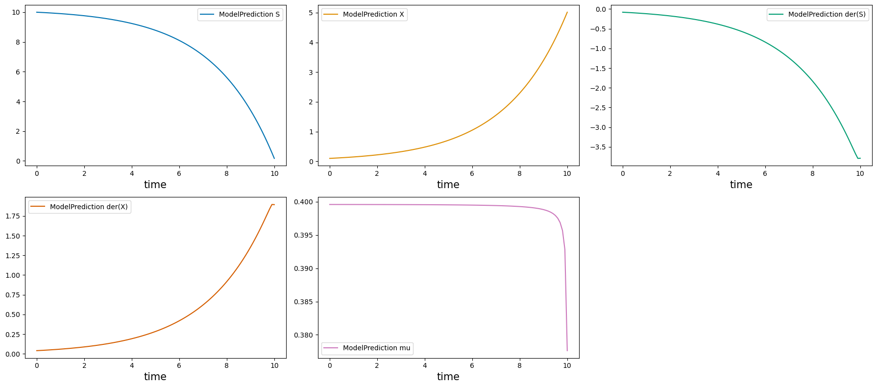
The method returns a Simulation object, which contains a list of ModelPredictions.

# simulation using default values and settings
simulation = SimpleBatchModel.simulate(
    t0= 0,
    t_end= 10,
    stepsize=0.1,
    )

_ = plot_simulation(simulation=simulation, observe=None)

../_images/e00fab7280ca61f6eaf45d47b89e03fab6496b0279d0ea7d60c5d78672d9f303.png

1. Modeling & Simulation

Contents