6. Monte Carlo Sampling#
With Monte Carlo sampling, also referred to as parametric bootstrap, the probabiliy distribution of model parameters is approximated by generating a large number of artificial measurements (resampling) and re-estimating model parameters for each.
For a detailed description of the method the interested reader is referred to:
Imports#
from estim8.models import FmuModel
from estim8 import visualization, datatypes, Estimator
from estim8.error_models import LinearErrorModel
import pandas as pd
6.1 Load the model#
SimpleBatchModel = FmuModel(path='../tests/test_data/SimpleBatch.fmu')
6.2 Import experimental data & create an Experiment object#
To quantify the extend at which uncertainty in experimental data propagates to parameter estimates, we need to define it first using a mathematical model.
Per default, estim8 assumes normally distributed measurement noise, e.g. using the LinearErrorModel (Notebook 2. Experimental data and error modeling).
data = pd.read_excel(r'SimpleBatch_Data.xlsx', index_col=0, header=(0, 1))
data.columns = data.columns.droplevel(1)
print(data.head())

# use a linear error model with normally distributed noise
experiment = datatypes.Experiment(data, error_model=LinearErrorModel(slope=0.05, offset=0.1))
Time         X   S
0.0   0.176200 NaN
0.1   0.318313 NaN
0.2   0.285270 NaN
0.3   0.218600 NaN
0.4   0.248210 NaN
6.3 Defining the estimation problem & create Estimator object#
As described in Notebook 3. Parameter estimation, unknown parameters and their bounds are defined and an Estimator instance is created.
## define unknown parameters with upper and lower bounds
bounds = {
    'X0': [0.05, 0.15],
    'mu_max': [0.1, 0.9],
    'Y_XS': [0.1, 1]
}

# create an estimator object
estimator = Estimator(
    model=SimpleBatchModel,
    bounds=bounds,
    data=experiment,
    t=[0, 10, 0.1],
    metric="negLL"
)
6.4 Start Monte Carlo Sampling#
Monte carlo sampling runs an optimization for each generated sample, therefore the method provides the same arguments and keyword arguments as a single estimation job using the Estimator’s estimate method:
Argument |
Type |
Description |
|---|---|---|
method |
str or List[str] |
the method key of the optimization algorithm. Pygmo algorithms are passed as a List[str] |
max_iter |
int |
maximum iteration rounds for the solver algorithm per estimation job. |
Kwarg |
Type |
Description |
n_jobs |
int |
number of parallel jobs to run the optimization algorithm with for each estimation job |
optimizer_kwargs |
dict |
Keyword arguments for the optimization function |
Additionall arguments and keyword arguments for the mc_sampling method are
Kwarg |
Type |
Description |
|---|---|---|
n_samples |
int |
The number of Monte Carlo samples |
mcs_at_once |
int |
number of Monte carlo estimations run in parallel |
optimizer_kwargs |
dict |
keyword arguments for the optimization function |
⚠️ This method puts considerable amount of work on your machine!
mc_samples = estimator.mc_sampling(
    method='de',
    max_iter=1000,      # maximum iterations for each estimation run
    n_jobs=1,           # parallelization of each estimation run
    mcs_at_once=6,      # number of Monte Carlo estimations to run in parallel
    n_samples=100       # number of monte carlo samples
)
---- Sample 1 completed
---- Sample 2 completed
---- Sample 3 completed
---- Sample 4 completed
---- Sample 5 completed
---- Sample 6 completed
---- Sample 7 completed
---- Sample 8 completed
---- Sample 9 completed
---- Sample 10 completed
---- Sample 11 completed
---- Sample 12 completed
---- Sample 13 completed
---- Sample 14 completed
---- Sample 15 completed
---- Sample 16 completed
---- Sample 17 completed
---- Sample 18 completed
---- Sample 19 completed
---- Sample 20 completed
---- Sample 21 completed
---- Sample 22 completed
---- Sample 23 completed
---- Sample 24 completed
---- Sample 25 completed
---- Sample 26 completed
---- Sample 27 completed
---- Sample 28 completed
---- Sample 29 completed
---- Sample 30 completed
---- Sample 31 completed
---- Sample 32 completed
---- Sample 33 completed
---- Sample 34 completed
---- Sample 35 completed
---- Sample 36 completed
---- Sample 37 completed
---- Sample 38 completed
---- Sample 39 completed
---- Sample 40 completed
---- Sample 41 completed
---- Sample 42 completed
---- Sample 43 completed
---- Sample 44 completed
---- Sample 45 completed
---- Sample 46 completed
---- Sample 47 completed
---- Sample 48 completed
---- Sample 49 completed
---- Sample 50 completed
---- Sample 51 completed
---- Sample 52 completed
---- Sample 53 completed
---- Sample 54 completed
---- Sample 55 completed
---- Sample 56 completed
---- Sample 57 completed
---- Sample 58 completed
---- Sample 59 completed
---- Sample 60 completed
---- Sample 61 completed
---- Sample 62 completed
---- Sample 63 completed
---- Sample 64 completed
---- Sample 65 completed
---- Sample 66 completed
---- Sample 67 completed
---- Sample 68 completed
---- Sample 69 completed
---- Sample 70 completed
---- Sample 71 completed
---- Sample 72 completed
---- Sample 73 completed
---- Sample 74 completed
---- Sample 75 completed
---- Sample 76 completed
---- Sample 77 completed
---- Sample 78 completed
---- Sample 79 completed
---- Sample 80 completed
---- Sample 81 completed
---- Sample 82 completed
---- Sample 83 completed
---- Sample 84 completed
---- Sample 85 completed
---- Sample 86 completed
---- Sample 87 completed
---- Sample 88 completed
---- Sample 89 completed
---- Sample 90 completed
---- Sample 91 completed
---- Sample 92 completed
---- Sample 93 completed
---- Sample 94 completed
---- Sample 95 completed
---- Sample 96 completed
---- Sample 97 completed
---- Sample 98 completed
---- Sample 99 completed
---- Sample 100 completed
6.5 Evaluation of Monte Carlo Sampling#
For further evaluation and saving the sampling results e.g. to an Excel-file, the Monte Carlo samples mc_samples are stored in a pandas.DataFrame. This dataframe can then be passed to the different evaluation plot methods provided by the visualization submodule.
samples = pd.DataFrame(data = [elem[0] for elem in mc_samples]) # extract the parameter - estimate dictionary frome each sample and create a pandas DataFrame
samples.index.name = 'sample'
samples.head()
| X0 | mu_max | Y_XS | |
|---|---|---|---|
| sample | |||
| 0 | 0.088772 | 0.515231 | 0.497925 |
| 1 | 0.098316 | 0.500571 | 0.492545 |
| 2 | 0.091886 | 0.511739 | 0.496357 |
| 3 | 0.086416 | 0.518745 | 0.496050 |
| 4 | 0.085875 | 0.521317 | 0.497505 |
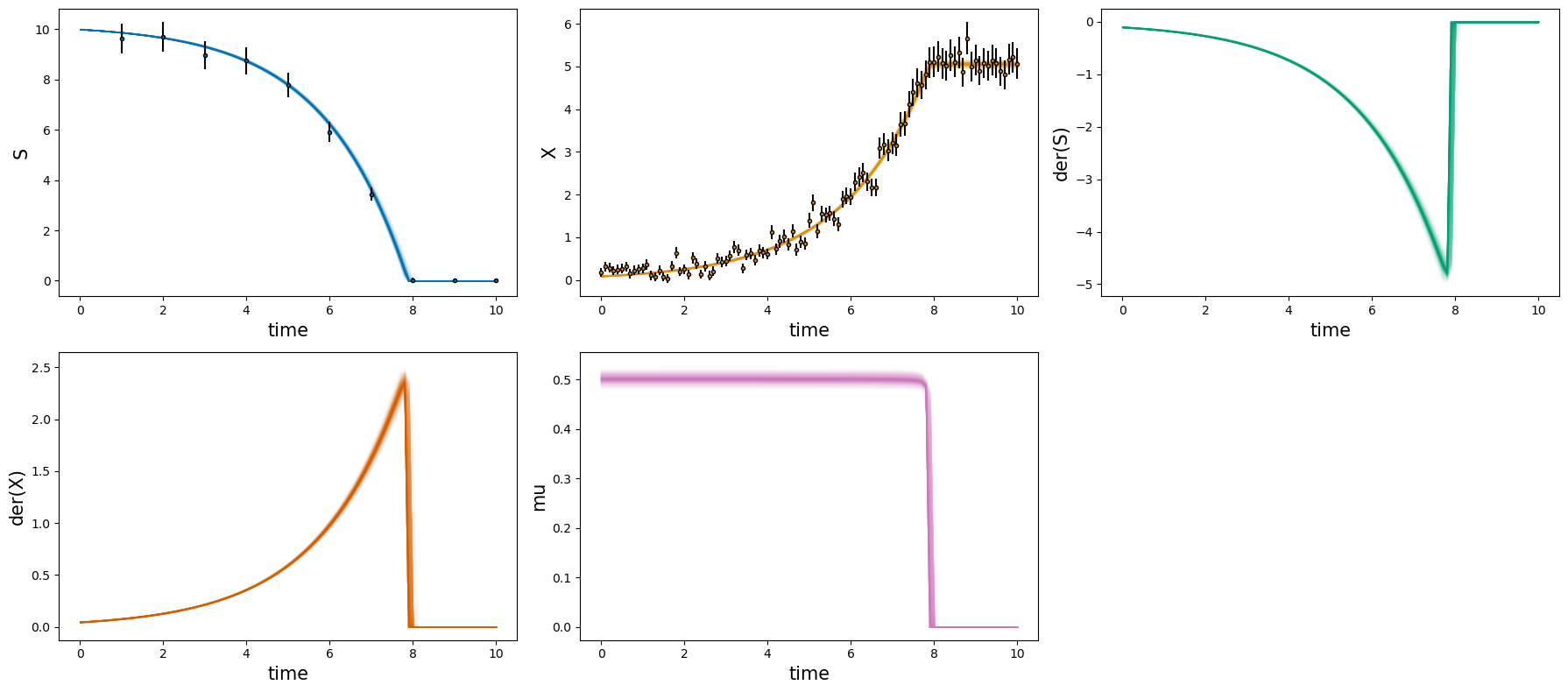
6.5.1 Forward simulation plot of Monte Carlo samples#
The first step when evaluating the sampling result should be a “posterior check”. For this matter, the plot_estimates method shows the density of resulting model predictions compared to experimental data.
# forward simulations
_ = visualization.plot_estimates_many(mc_samples=samples, estimator=estimator)
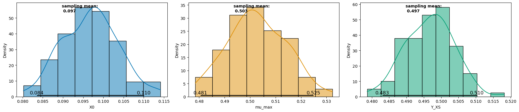
6.5.2 Parameter distributions#
The plot_distributions method can then be used to plot the parameter distributions via histograms along with statistical metrics of sampling mean and confidence interval ( 95 % in the example below).
_ = visualization.plot_distributions(samples, ci_level=0.95)
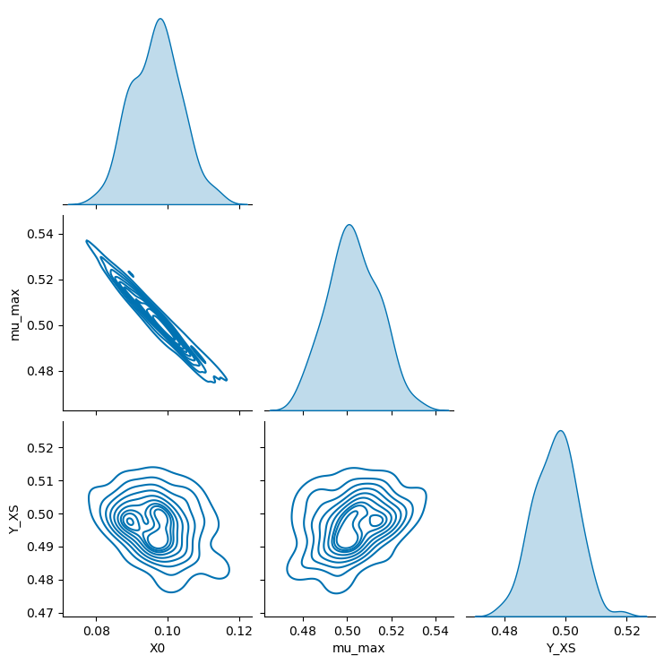
6.5.3 Pair plots#
Finally, parameter correlations can be revealed using the plot_pairs method.
_ = visualization.plot_pairs(samples, kind="kde")