3. Parameter estimation

This notebook introduces the Estimator class and demonstrates it’s functions for paramater estimation using the example of a simple batch model (see Notebook 1. Modeling & Simulation).

Import dependencies

from estim8.models import FmuModel
from estim8 import visualization, datatypes, Estimator, generalized_islands
import pandas as pd
import pygmo

1. Load the SimpleBatch FMU model

SimpleBatchModel = FmuModel(path=r'../tests/test_data/SimpleBatch.fmu')
print(f"Model parameters: \n {SimpleBatchModel.parameters}")
print(f"Model observables: \n {SimpleBatchModel.observables}")

Model parameters: 
 {'Ks': 0.01, 'S0': 10.0, 'X0': 0.2, 'Y_XS': 0.35, 'mu_max': 0.4}
Model observables: 
 ['S', 'X', 'der(S)', 'der(X)', 'mu']

2. Load experimental data & datastructure setup

In order to setup an Experiment datastructure (see Notebook 2), raw measurement data is loaded first. Here, the function pandas.read_excel is used to read the contents of an Excel sheet SimpleBatch_Data.xlsx, which contains artificial measurements for biomass concentration X \([g \cdot L^{-1}]\) and substrate concentration S \([g \cdot L^{-1}]\) over the duration of a batch cultivation.

# import datasheet
data = pd.read_excel(r'SimpleBatch_Data.xlsx', index_col=0, header=(0,1))
data.head(11)

Time	X	S
h	g/L	g/L
0.0	0.176200	NaN
0.1	0.318313	NaN
0.2	0.285270	NaN
0.3	0.218600	NaN
0.4	0.248210	NaN
0.5	0.268477	NaN
0.6	0.312500	NaN
0.7	0.150687	NaN
0.8	0.226870	NaN
0.9	0.258150	NaN
1.0	0.275126	9.632284

Before creating an Experiment object by passing the created DataFrame, the multi-index must be removed.

For this simple example no we assume the Experiment’s default LinearErrorModel to describe the noises of Measurements (see Notebook 2. Experimental data and error modeling). As the names of the columns in data directly correspond to the states in SimpleBatchModel.observables no observation_mapping must be defined.

# drop the multi-index header and show resulting dataframe
data.columns = data.columns.droplevel(1)
display(data)

# create an Experiment object
experiment = datatypes.Experiment(data) 

Time	X	S
0.0	0.176200	NaN
0.1	0.318313	NaN
0.2	0.285270	NaN
0.3	0.218600	NaN
0.4	0.248210	NaN
...	...	...
9.6	4.885956	NaN
9.7	4.807351	NaN
9.8	5.167874	NaN
9.9	5.220779	NaN
10.0	5.065959	0.0

101 rows × 2 columns

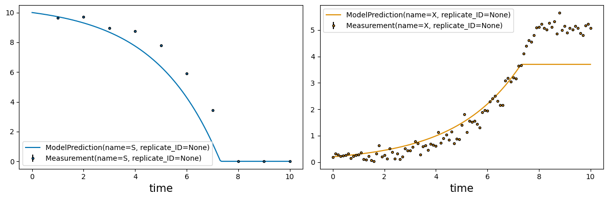
To compare the unfitted model’s precitions to experimental data, the plot_simulation function of the visualization submodule takes a keyword argument experiment.

# compare simulation to data
simulation = SimpleBatchModel.simulate(t0=0, t_end=10, stepsize=0.1)
_ = visualization.plot_simulation(simulation=simulation, experiment=experiment, observe=['S', 'X'])

3. Problem definition

Besides a model for forward simulation and experimental data, an estimation problem is defined by unknown parameters and and their bounds using a dictionary.

## define unknown parameters with upper and lower bounds
bounds = {
    'X0': [0.05, 0.15],
    'mu_max': [0.1, 0.9],
    'Y_XS': [0.1, 1]
}

4. The Estimator class

The Estimator class collects all single parts of a problem defined by the user and manages the processes of model fitting. Creating an instance of this class requires the following arguments:

Argument	Type	Description
model	models.Estim8Model	The model class to be fitted. Must be a subclass of Estim8Model that runs the simulations.
bounds	dict[str, List[float]]	Dictionary defining the parameter bounds for estimation. Format: {“param_name”: [lower_bound, upper_bound]}.
data	Experiment | Dict[str, Experiment]	Experimental data for model fitting. Can be single experiment or multiple replicates as Experiment objects in form of dict{replicate_ID: Experiment}.

Optional keyword arguments are:

Kwarg	Type	Description
t	List[float], optional	Time vector specification as [t_0, t_end, step_size]. If None, will be automatically determined from the experimental data
metric	Literal[“SS”, “WSS”, “negLL”], optional	Loss function for optimization: “SS” (Sum of squared residuals), “WSS” (Weighted sum of squared residuals), or “negLL” (Negative log-likelihood). Default is “SS”
parameter_mapping	List[ParameterMapper] | ParameterMapping, optional	Defines parameter relationships between replicates. Can be list of mappings or complete ParameterMapping object. None means all parameters applied to all model replicates (default)

# Instantiating an Estimator object
estimator = Estimator(
    model=SimpleBatchModel,     # model used for simulation
    bounds=bounds,              # unknown parameters and bounds
    data=experiment,            # experimental data
    t=[0, 10, 0.1],             # the timeframe for model simulation as [t_0, t_end, step_size],
    metric = 'SS'               # default objective function Sum of squared residuals
)

4.1 Parameter estimation

Estim8 supports a variety of optimzation algorithms from scipy.optimize, scikit-optimize and pygmo. Is is higly recommended to check out their documentations, e.g. for the use of solver hyperparameters and keyword arguments.

The optimization algorithm of choice is specified by passing a corresponding method key to the function Estimator.estimate.

4.1.1 scipy and scikit-optimize alogorithms and keys:

Method key	Optimization function	Solver parallelization
local	scipy.optimize.minimize	❌
de	scipy.optimize.differential_evolution	✅
bh	scipy.optimize.basinhopping	❌
shgo	scipy.optimize.shgo	✅
dual_annealing	scipy.optimize.dual_annealing	❌
gp	skopt.gp_minimize	✅

In this example, the differential_evolution function from scipy.optimize is used to solve the estimation problem.

The estimation is started by calling the function Estimator.estimate. It takes at least the following arguments:

Argument	Type	Description
method	str or List[str]	the method key of the optimization algorithm. Pygmo algorithms are passed as a List[str] (see below).
max_iter	int	maximum iteration rounds for the solver algorithm

Additionally, keyword arguments include:

Kwarg	Type	Description
n_jobs	int	number of parallel jobs to run the optimization algorithm with.
optimizer_kwargs	dict	keyword arguments for the optimization function

Finally, the Estimator.estimate method returns the estimated parameters and an info-object containing additional information about the optimization procedure.

estimates, info = estimator.estimate(
    method              =   'de',           # method key of the optimization algorithm
    max_iter            =   1000,           # maximum number of iterations for the solver
    n_jobs              =   1,              # process pool size of the solver algorithm     
    optimizer_kwargs    =   {               # kewyword arguments to pass to the differential_evolution function:
                'disp': True,               # prints the evolution process
                "x0": [0.15, 0.3, 0.4],     # initial guess for the unknown parameters
                "popsize": 15,              # population size
            }
)

print(f" \nEstimated parameters: \n{estimates}")
print(f"Estimation info: \n{info}")

differential_evolution step 1: f(x)= 12.684329880089283
differential_evolution step 2: f(x)= 11.706434145847094
differential_evolution step 3: f(x)= 6.777913020490919
differential_evolution step 4: f(x)= 6.777913020490919
differential_evolution step 5: f(x)= 4.518898563207684
differential_evolution step 6: f(x)= 4.146746395520315
differential_evolution step 7: f(x)= 4.146746395520315
differential_evolution step 8: f(x)= 4.146746395520315
differential_evolution step 9: f(x)= 4.015157178278605
differential_evolution step 10: f(x)= 4.015157178278605
differential_evolution step 11: f(x)= 4.015157178278605
differential_evolution step 12: f(x)= 4.015157178278605
differential_evolution step 13: f(x)= 4.015157178278605
differential_evolution step 14: f(x)= 4.010950571057011
differential_evolution step 15: f(x)= 3.875815230688865
differential_evolution step 16: f(x)= 3.875815230688865
differential_evolution step 17: f(x)= 3.8539449971522846
differential_evolution step 18: f(x)= 3.8539449971522846
differential_evolution step 19: f(x)= 3.853532152759052
differential_evolution step 20: f(x)= 3.853532152759052
differential_evolution step 21: f(x)= 3.8517063088344847
differential_evolution step 22: f(x)= 3.850866803681322
Polishing solution with 'L-BFGS-B'
 
Estimated parameters: 
{'X0': 0.10397303940339815, 'mu_max': 0.49402848576448555, 'Y_XS': 0.4987637416997156}
Estimation info: 
             message: Optimization terminated successfully.
             success: True
                 fun: 3.850866803681322
                   x: [ 1.040e-01  4.940e-01  4.988e-01]
                 nit: 22
                nfev: 1231
          population: [[ 1.040e-01  4.940e-01  4.988e-01]
                       [ 1.032e-01  4.942e-01  5.017e-01]
                       ...
                       [ 9.719e-02  5.021e-01  4.988e-01]
                       [ 1.049e-01  4.941e-01  5.008e-01]]
 population_energies: [ 3.851e+00  3.894e+00 ...  3.913e+00  3.889e+00]

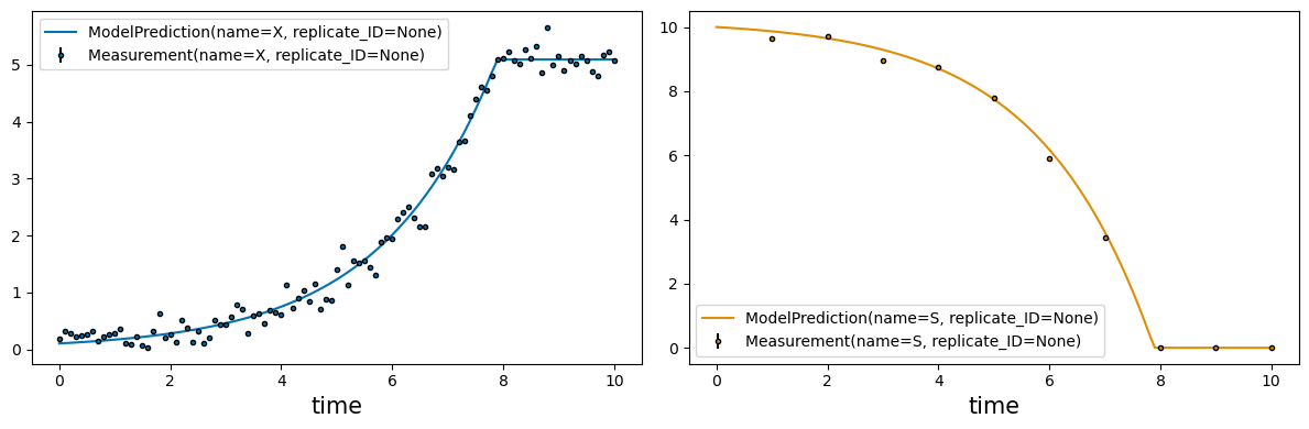
Visualizing estimation results

To inspect the optimization results. the plot_estimates function from the visualization submodule convenient plots:

# compare fitted model to data
_ = visualization.plot_estimates(estimates=estimates, estimator=estimator, only_measured=True)

4.1.2 Parallelized parameter estimation

In many cases the parameter estimation time can be reduced by parallelizing the optimization function using multiple CPUs. In this example, 4 parallel jobs are used for the differential evolution algorithm by setting n_jobs=4 when calling the estimate function:

estimates, info = estimator.estimate(
    method              =   'de',           # method key of the optimization algorithm
    max_iter            =   1000,           # maximum number of iterations for the solver
    n_jobs              =   4,              # process pool size of the solver algorithm     
    optimizer_kwargs    =   {               # kewyword arguments to pass to the differential_evolution function:
                'disp': True,               # prints the evolution process
                "x0": [0.15, 0.3, 0.4],     # initial guess for the unknown parameters in the same order as unknowns
                "popsize": 15,              # population size
            }
)

c:\Users\Tobia\miniforge-pypy3\envs\testim8\lib\site-packages\scipy\optimize\_differentialevolution.py:487: UserWarning: differential_evolution: the 'workers' keyword has overridden updating='immediate' to updating='deferred'
  with DifferentialEvolutionSolver(func, bounds, args=args,

differential_evolution step 1: f(x)= 12.052963396189778
differential_evolution step 2: f(x)= 7.866859773792932
differential_evolution step 3: f(x)= 6.703361312953871
differential_evolution step 4: f(x)= 6.703361312953871
differential_evolution step 5: f(x)= 5.316231351946375
differential_evolution step 6: f(x)= 3.9258677107470934
differential_evolution step 7: f(x)= 3.9258677107470934
differential_evolution step 8: f(x)= 3.9258677107470934
differential_evolution step 9: f(x)= 3.9258677107470934
differential_evolution step 10: f(x)= 3.9258677107470934
differential_evolution step 11: f(x)= 3.9258677107470934
differential_evolution step 12: f(x)= 3.9258677107470934
differential_evolution step 13: f(x)= 3.9258677107470934
differential_evolution step 14: f(x)= 3.9258677107470934
differential_evolution step 15: f(x)= 3.9258677107470934
differential_evolution step 16: f(x)= 3.9052917277289216
differential_evolution step 17: f(x)= 3.9005841453150882
differential_evolution step 18: f(x)= 3.9005841453150882
differential_evolution step 19: f(x)= 3.9005841453150882
differential_evolution step 20: f(x)= 3.8940172609612604
differential_evolution step 21: f(x)= 3.8628508279319425
differential_evolution step 22: f(x)= 3.8553200609239426
differential_evolution step 23: f(x)= 3.8553200609239426
differential_evolution step 24: f(x)= 3.8553200609239426
differential_evolution step 25: f(x)= 3.8553200609239426
differential_evolution step 26: f(x)= 3.853163942552897
differential_evolution step 27: f(x)= 3.849826555357635
differential_evolution step 28: f(x)= 3.849826555357635
Polishing solution with 'L-BFGS-B'

4.2 Advanced parameter estimation with pygmo

pygmo is a scientific Python library for massively parallel optimization, implementing a range of state-of-the-art bio-inspired and evolutionary algorithms. Using the asynchronous, generalized islands model, these algorithms can be easily mixed via a topology, yielding a “super algorithm” that exploits algorithmic cooperation. estim8 features the following algorithms:

method key	algorithm
scipy_optimize	A wrapper around scipy.optimize.minimize
de1220	Self-adaptive Differential Evolution, pygmo flavour (pDE)
bee_colony	Artificial Bee Colony
gaco	Extended Ant Colony Optimization algorithm
pso	Particle Swarm Optimization
sga	A Simple Genetic Algorithm
sea	(N+1)-ES simple evolutionary algorithm
compass_search	Compass Search
gwo	Grey Wolf Optimizer (gwo)
cmaes	Covariance Matrix Evolutionary Strategy (CMA-ES)
simulated_annealing	Simulated Annealing (Corana’s version)
nsga2	Non dominated Sorting Genetic Algorithm (NSGA-II)
mbh	Monotonic Basin Hopping (generalized)
ihs	Improved harmony search algorithm
xnes	Exponential Evolution Strategies
de	Differential Evolution

For using pygmo’s Generalized Islands approach, the estimate function is called with a list of algorithms keys in the method argument. A list of implemented topologies can be found here.

# algorithms for islands in heterogenous archipelago and keyword arguments (see pygmo documentation for more details)
algorithms_and_kwargs = {
    'sga'   : dict(gen=10, cr=.90, eta_c=1., m=0.02, param_m=1., param_s=2, crossover='exponential', mutation='polynomial', selection='tournament', seed=42),
    'pso'   : dict(gen=10, omega=0.7298, eta1=2.05, eta2=2.05, max_vel=0.5, variant=5, neighb_type=2, neighb_param=4, memory=False, seed=42),
    'de1220': dict(gen=10, allowed_variants=[2, 3, 7, 10, 13, 14, 15, 16], variant_adptv=1, ftol=1e-6, xtol=1e-6, memory=False, seed=42),
    'sea'   : {}    # here we use the default kwargs listed above
    }

# print the default algorithm kwargs for pygmo.sea algorithm
print(f"Default kwargs for pygmo.sea: {generalized_islands.PygmoHelpers.algo_default_kwargs['sea']} \n")


estimates_1, info_1 = estimator.estimate(   
    method = list(algorithms_and_kwargs.keys()),                # a list of algorithm keys defined above
    n_jobs=6,                                                   # process pool size of the solver algorithm
    max_iter=5,                                                # number of evolutions
    optimizer_kwargs = {
        'pop_size'      :   30,                                     # population size of each island
        'algos_kwargs'  :   list(algorithms_and_kwargs.values()),   # algorithm kwargs
        'topology'      :   pygmo.fully_connected(),                           # the archipelagos topology, default is pygmo.fully_connected()
        'report'        :   2                                       # prints out progress during evolutions and collects a trace of each island champion per evolution
    }
)

Default kwargs for pygmo.sea: {'gen': 40} 

[Parallel(n_jobs=4)]: Using backend LokyBackend with 4 concurrent workers.
[Parallel(n_jobs=4)]: Done   4 out of   4 | elapsed:    7.3s finished

>>> Created Island 1 using <pygmo.core.sga object at 0x000002A051CBCEF0>
>>> Created Island 2 using <pygmo.core.pso object at 0x000002A051CC6AF0>
>>> Created Island 3 using <pygmo.core.de1220 object at 0x000002A0516F5770>
>>> Created Island 4 using <pygmo.core.sea object at 0x000002A051CC4EB0>

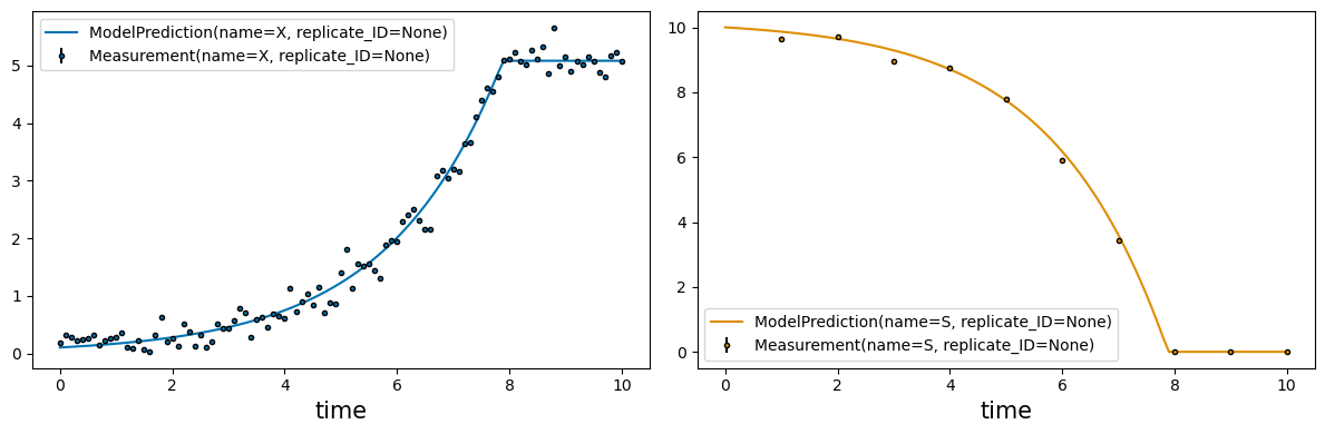
# compare fitted model to data
_ = visualization.plot_estimates(estimates=estimates, estimator=estimator, only_measured=True)

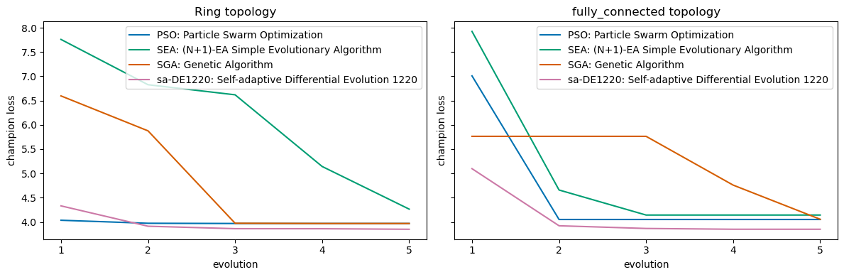
When calling the estimate function with report>=1, the info object provides an attribute evo_trace which is a pandas.DataFrame with data about the archipelago’s evolutions. This is usefull e.g. when comparing the performance of different algorithms or the archipelago’s topology setup.

In the following example a second approach using the same algorithms but fully unconnected islands (topology: pygmo.fully_connected()) is used for optimization. The evoltion traces of both approaches are then compared:

## 2. Archipelago optimization with unconnected islands
estimates_2, info_2 = estimator.estimate(   
    method = list(algorithms_and_kwargs.keys()),                # a list of algorithm keys defined above
    n_jobs=6,                                                   # process pool size of the solver algorithm
    max_iter=5,                                                # number of evolutions
    optimizer_kwargs = {
        'pop_size'      :   30,                                     # population size of each island
        'algos_kwargs'  :   list(algorithms_and_kwargs.values()),   # algorithm kwargs
        'topology'      :   pygmo.unconnected(),                    # run with unconnected islands
        'report'        :   1                                       # collects a trace of each island champion per evolution
    }
)

[Parallel(n_jobs=4)]: Using backend LokyBackend with 4 concurrent workers.
[Parallel(n_jobs=4)]: Done   2 out of   4 | elapsed:    7.6s remaining:    7.6s
[Parallel(n_jobs=4)]: Done   4 out of   4 | elapsed:    7.7s finished

>>> Created Island 1 using <pygmo.core.sga object at 0x000002A051EFE030>
>>> Created Island 2 using <pygmo.core.pso object at 0x000002A051CC22F0>
>>> Created Island 3 using <pygmo.core.de1220 object at 0x000002A051C67EF0>
>>> Created Island 4 using <pygmo.core.sea object at 0x000002A051CC23B0>

# plot the evolution traces of both approaches
import matplotlib.pyplot as plt
fig, axes = plt.subplots(1, 2, figsize=(12, 4), sharey=True)

for ax, info in zip(axes, [info_1, info_2]):
    islands_traces = info.evo_trace.groupby("algorithm")
    for group in islands_traces.groups:
        data = islands_traces.get_group(group)
        ax.plot(data.index.get_level_values("evolution"), data["champion_loss"], label=group)

    ax.set_xlabel("evolution")
    ax.set_ylabel("champion loss")
    ax.set_xticks(data.index.get_level_values("evolution"))
    ax.legend()

axes[0].set_title("Ring topology")
axes[1].set_title("fully_connected topology")

fig.tight_layout()

Continuing an estimation with pygmo

In case the number of evolutions turns out insufficient, the optimization of the archipelago can be continued by simply running estimate(method=info ..) using the info object returned by the preceeding estimation:

estimates, info = estimator.estimate(
    method      =   info_1,
    max_iter    =   5,          # run 5 more evolutions
)