2 Experimental data handling

This notebook introduces the functions and datatypes used in estim8 when working with experimental data. It covers the following topics:

• creating Measurement and Experiment objects for custom problems

• observation mapping

• error modeling

from estim8 import visualization, datatypes
import pandas as pd
import numpy as np
import matplotlib.pyplot as plt

# load data 
data = pd.read_excel('SimpleBatch_Data.xlsx', index_col=0, header=(0, 1))
data.head()

Time	X	S
h	g/L	g/L
0.0	0.176200	NaN
0.1	0.318313	NaN
0.2	0.285270	NaN
0.3	0.218600	NaN
0.4	0.248210	NaN

2.1 Experiments & Measurements

In estim8 the data is structured in Experiment objects, which consist of individual Measurement objects.

# drop multiindex header
data.columns = data.columns.droplevel(1)
exp = datatypes.Experiment(data)
exp.measurements

[Measurement(name=X, replicate_ID=None),
 Measurement(name=S, replicate_ID=None)]

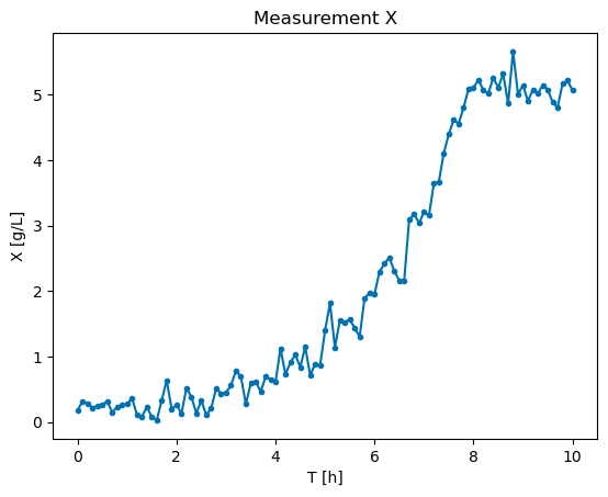
plt.plot( exp['X'].timepoints, exp['X'].values, marker=".")
plt.title('Measurement X')
plt.xlabel('T [h]')
plt.ylabel('X [g/L]')

Text(0, 0.5, 'X [g/L]')

An Experiment can also be created by passing defined Measurement objects:

# create measurement objects
measurements = [
    datatypes.Measurement(
        name=column, 
        timepoints=data.index,
        values=data[column].values
    )
    for column in data.columns
]

# create Experiment bbject
exp = datatypes.Experiment(measurements=measurements)

2.2 Observation mappings

To map specific measurements to model states with different names, one can define an observation mapping.

# create a dataframe with different names
df = data.copy()
df.columns= ['obs_X', 'obs_S']
display(df.head())

# define an observation mapping
observation_mapping = {
#   measurement:    model
    'obs_X':        'X',
    'obs_S':        'S'
}

exp = datatypes.Experiment(df, observation_mapping = observation_mapping)

	obs_X	obs_S
0.0	0.176200	NaN
0.1	0.318313	NaN
0.2	0.285270	NaN
0.3	0.218600	NaN
0.4	0.248210	NaN

2.3 Error modeling

In objective functions like the weighted sum of squared residuals (WSS) or negative Log-likelihood (negLL) we use the measurement noise \(\sigma\) as weights when quantifying model discrepancy.

2.3.1 Linear error model

Per default, estim8 uses a linear error model, which describes the noise as

\[ \begin{align} \sigma_i = slope \cdot y_{i_{measured}} + offset \end{align} \]

where slope and offset refer to the relative and absolute error respectively.

from estim8.error_models import LinearErrorModel

# create a error model instance
my_error_model = LinearErrorModel(slope=0.05, offset=0.01)

# pass the error model to the experiment, which will pass it further to individual measurements
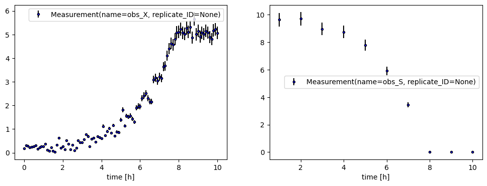
exp = datatypes.Experiment(df, error_model=my_error_model)

# plot measurement with errorbars
fig, axes = plt.subplots(1,2, figsize=(12,4))
for ax, measurement in zip(axes, exp.measurements):
    visualization.plot_measurement(ax=ax, measurement=measurement, color='blue')
    ax.set_xlabel("time [h]")
    ax.legend()

2.3.2 Measurement-specific error models

# create an error model instance with an absolute error only e.g. fo a specific measurement
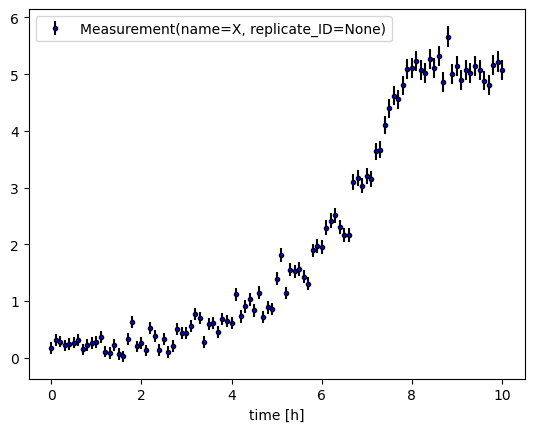
error_model_X = LinearErrorModel(slope=0, offset=0.2)

# create a measurement object with unique error model
measurement_X = datatypes.Measurement(
    name='X',
    timepoints=data.index,
    values=data['X'].values,
    error_model=error_model_X
)

# plot measurement with errorbars
fig, ax = plt.subplots()
_ = visualization.plot_measurement(ax=ax, measurement=measurement_X, color='blue')
ax.set_xlabel('Time [h]')
ax.legend()

<matplotlib.legend.Legend at 0x199277c6ef0>

Alternatively, one can always provide an array of error values when creating a Measurement object.

# create an array of error values with same shape as measurement values
errors = np.ones_like(data['X'].values)*0.4

meas = datatypes.Measurement(
    name='X',
    timepoints=data.index,
    values=data['X'].values,
    errors=errors
)

# plot the measurement with errors
_, ax = plt.subplots()
visualization.plot_measurement(ax=ax, measurement=meas, color='blue')
ax.legend()
ax.set_xlabel('time [h]')

Text(0.5, 0, 'time [h]')

2.3.3 Custom error models

Own error model classes can be easily implemented by inheriting from estim8’s base class BaseErrorModel. The custom class implementation should at least have the class method generate_error_data, which recieves a numpy.ndarray of datapoints and returns an array of errors.

from scipy.stats.distributions import norm, rv_continuous
from estim8.error_models import BaseErrorModel

class PoylnomialErrorModel(BaseErrorModel):

    def __init__(self, a,b,c):
        self.a = a 
        self.b = b
        self.c = c
        super().__init__()
    

    def generate_error_data(self, values: np.array) -> np.array:
        return self.a * values **2 + self.b * values + self.c
    

# create an instance of PolynomialErrorModel
polynomialErrorModel = PoylnomialErrorModel(
    a=1e-3,
    b=1e-2,
    c=1e-1
)

# create a Measurement object, passing the custom error model
meas = datatypes.Measurement(
    name = 'X',
    values = data['X'].values,
    timepoints=data.index,
    error_model=polynomialErrorModel

)

# plot the measurement with errors
_, ax = plt.subplots()
visualization.plot_measurement(ax=ax, measurement=meas, color='blue')
ax.legend()
ax.set_xlabel('time [h]')

Text(0.5, 0, 'time [h]')

2.4 Error distributions

Uncertainty quantification techniques like profile likelihoods (see Notebook 5) and Monte Carlo sampling (see Notebook 6) or calculations of a statistical likelihood require modeling the data via distributions.

2.4.1 Basics on likelihood and data distribution

For likelihood driven objectives such as the negLL function, the data is described via a probability distribution. In many cases it is assumed that the data is normally distributed. Parametrized by mean \(\hat{y}\) and standard deviation \(\sigma\), the probability density function (PDF) follows

$

(1)\[\begin{align} PDF(y)= \frac{1}{\sqrt{2 \pi \sigma^2}} \cdot e^{- \frac{(y-\hat{y})^2}{2 \sigma^2}} \end{align}\]

$

Per default, estim8’s ErrorModel use a normal distribution. For the first datapoint of the biomass measurements X from above e.g., the likelihood \(p\) of the data \(y\) given a model prediction \(y_{model}\) is determined by evaluating \(pdf(y_{model})\):

meas = datatypes.Measurement(
    name='X',
    timepoints=data.index,
    values=data['X'].values,
    error_model= LinearErrorModel(slope=0, offset=0.05) # we use an absolute error model with sigma=0.05 for every datapoint
)

# get the first datapoint
y_hat = meas.values[0]
sigma = meas.errors[0]

# create array of some possibl values for y
y_model_range = np.linspace(max(0,y_hat-6*sigma), y_hat+6*sigma, 100)
likelihood_y_model_range = meas.error_model.error_distribution.pdf(x=y_model_range, loc=y_hat, scale=sigma)
# plot the pdf for the y range
plt.plot(y_model_range,likelihood_y_model_range )
plt.fill_between(y_model_range, y1=np.zeros_like(y_model_range), y2=likelihood_y_model_range, alpha=0.1, color='blue')
pdf_y_hat = meas.error_model.error_distribution.pdf(x=y_hat, loc=y_hat, scale=sigma)


# define a "simulated" model prediction for y
y_model = y_hat-1.6*sigma
likelihood_y_model = meas.error_model.error_distribution.pdf(x=y_model, loc=y_hat, scale=sigma)

# plot y_hat
plt.vlines(x=y_hat, ymin=0, ymax=pdf_y_hat, linestyles='dashed', colors='green')
plt.annotate(r"$\hat{y}$="+str(y_hat), xy=(y_hat*1.1, pdf_y_hat/2), color='green')
# plot sigma
plt.hlines(y=0, xmin=y_hat, xmax=y_hat+sigma, linestyles='dashed', color='orange')
plt.annotate(r"$\sigma$="+str(sigma),xy=(y_hat+(sigma/2), 0.1),color='orange')


# plot likelihoood of model prediction
plt.vlines(x=y_model, ymax=likelihood_y_model, ymin=0, color='red', linestyles="dashed")
plt.hlines(y=likelihood_y_model, xmin=min(y_model_range), xmax=y_model, colors='red',linestyles='dashed')
plt.annotate(r'$y_{model}$', xy=(y_model*1.1, likelihood_y_model/2), color='red')
plt.annotate(r"$p(y|y_{model},\sigma)$", xy=(y_model/2, likelihood_y_model*1.1), color='red')

plt.xlabel('y')
plt.ylabel('PDF(y)')
plt.title(r"Likelihood of model prediction $y_{model} \; given \; normally \; distributed \; data$")
fig.tight_layout()

2.4.2 Working with custom error distributions

In order to use different or completely customized error distributions, a distribution instance (a subclass of scipy.stats.rv_continuous ) can be passed when creating an error model object. For an overview of available continuous distributions, check out the docs of scipy.

In the example below, the student t distribution is used, which additionally takes a parameter df as input:

from scipy.stats import rv_continuous, t

err_model = LinearErrorModel(
    slope=0, 
    offset=0.05,
    error_distribution=t,
    error_distribution_kwargs={'df':10}
)