5 Parameter Identifiability - Profile Likelihoods

This notebook demonstrates how to evaluate parameter identifiability and to derive Confidence Intervals using profile likelihoods, a technique to analyse structural and practical identifiability of model parameters. In estim8, this procedure samples the likelihood profile of a parameter of interest by fixing it at certain values and then re-estimating the remaining free parameters.

For the interested reader the following references provide an in-depth discussion of the method:

• A. Raue, C. Kreutz, T. Maiwald, J. Bachmann, M. Schilling, U. Klingmüller, J. Timmer, Structural and practical identifiability analysis of partially observed dynamical models by exploiting the profile likelihood, Bioinformatics, Volume 25, Issue 15, August 2009, Pages 1923–1929, https://doi.org/10.1093/bioinformatics/btp358

• Kreutz C, Raue A, Kaschek D, Timmer J. Profile likelihood in systems biology. FEBS J. 2013 Jun;280(11):2564-71. doi: 10.1111/febs.12276. Epub 2013 May 9. PMID: 23581573.

from estim8.models import FmuModel
from estim8 import visualization, datatypes, Estimator
from estim8.error_models import LinearErrorModel
from estim8.profile import approximate_confidence_interval, calculate_negll_thresshold
import pandas as pd
import matplotlib.pyplot as plt

5.1 Load the model

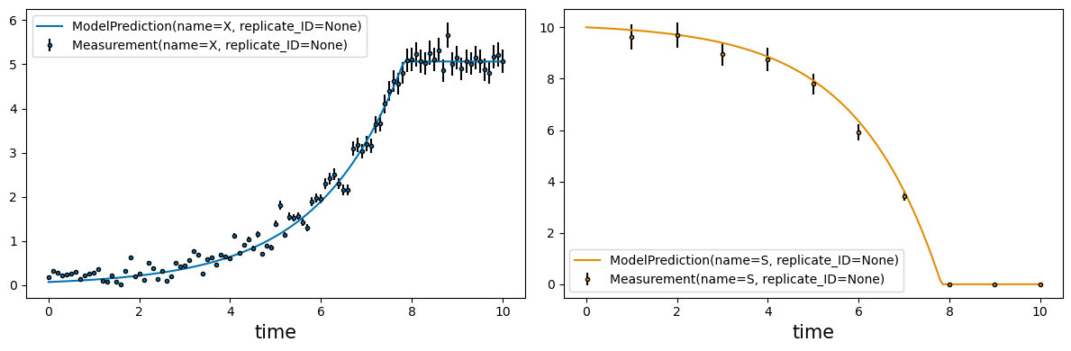
For demonstration purpose, the SimpleBatch model introduced in Notebook 1. Modeling & Simulation is used.

SimpleBatchModel = FmuModel(path='../../../tests/test_data/SimpleBatch.fmu')

# run a simulation with default parameters
simulation = SimpleBatchModel.simulate(t0=0, t_end=10, stepsize=1e-3, observe=["X", "S"])
_ = visualization.plot_simulation(simulation)

5.2 Import experimental data

The profile likelihood method translates the uncertainty in experimental data to model parameters. It is therefore a likleihood-driven techniqe which requires to model the data with some sort of probability distribution. In this example and in many real world problems, the measurement noise is assumed to be normally distributed, which is the default in estim8’s LinearErrorModel:

data = pd.read_excel(r'SimpleBatch_Data.xlsx', index_col=0, header=(0, 1))
data.columns = data.columns.droplevel(1)
data.head()

# assume a linear error model with relative error (scale) of 5% and an absolute error (offset) of 0.01
error_model = LinearErrorModel(
    slope=0.05,
    offset=0.01,
    )
# print the error models error distribution
print(error_model.error_distribution.__class__)

# create an experiment object
experiment = datatypes.Experiment(
    measurements=data,
    error_model=error_model,
    )

<class 'scipy.stats._continuous_distns.norm_gen'>

5.3 Defining the estimation problem & create Estimator object

Like in Notebook 3. Parameter estimation, the estimation problem is defined with unknown model parameters and their bounds. The Estimator class then serves as a central hub to collect all inputs and to manage parameter estimations.

## define unknown parameters with upper and lower bounds
bounds = {
    'X0': [0.05, 0.15],
    'mu_max': [0.1, 0.9],
    'Y_XS': [0.1, 1]
}

estimator = Estimator(
    model=SimpleBatchModel,
    bounds=bounds,
    data=experiment,
    t=[0, 10, 0.1],
    metric="negLL"      # use tthe negative log likelihood as the objective function
)

5.4 Find the Optimum

The estimate method is then used to obtain point estimators.

estimates, est_info = estimator.estimate(
    method='de',
    max_iter=1000,
    n_jobs=4,
    optimizer_kwargs={
        "tol": 1e-3
    }
)

_ = visualization.plot_estimates(estimator=estimator, estimates=estimates, only_measured=True)

c:\Users\Latour\AppData\Local\miniforge3\envs\testim8\Lib\site-packages\scipy\optimize\_differentialevolution.py:487: UserWarning: differential_evolution: the 'workers' keyword has overridden updating='immediate' to updating='deferred'
  with DifferentialEvolutionSolver(func, bounds, args=args,

5.5 Profile Likelihood Calculation

The Estimator’s profile_likelihood function is then used to sample the profiles likelihoods using a sampler with a fixed stepsize in descending/ascending direction from the estimated optimum for each parameter of interest. As this is a technique based on re-estimation, the same arguments for a single parameter estimation task described in Notebook 3. Parameter estimation can be used. The function takes at least the following arguments:

Arg	Type	Description
p_opt	dict	The estimated optimal parameters
method	str | List[str]	The optimization method(s) to use for each estimation job
max_iter	int	Maximum number of iterations for each optimization
n_jobs	int	Parallelization of each individual estimation

Key-word arguments comprise:

Kwarg	Type	Description
optimizer_kwargs	dict	Additional arguments passed to the optimization function
p_at_once	int	Number of parallel profile samplers at once. Default is 1
alpha	float	Confidence level of the profile likleihood, default is 0.05.
max_points	int	Maximum number of grid points to evaluate per parameter and direction. Default is None, in which case each sampler proceeds until a negLL threshold based upon a \(\chi^2\) quantile given alpha is reached.
stepsize	float	Relative parameter variation stepsize (between 0 and 1) for each parameter, default is 0.02
p_inv	list	List of parameters to investigate (defaults to all parameters in p_opt)

⚠️ This method puts considerable amount of work on your machine!

pl_result = estimator.profile_likelihood(
    p_opt= estimates,
    # arguments for each estimation procedure    
    method='de',
    optimizer_kwargs={
        "tol": 1e-3
    },        
    max_iter=1000,       
    n_jobs=1,
    # profiling arguments           
    p_at_once=6,         
    stepsize=0.006,      
)

5.6 Evaluation of profile likelihoods

5.6.1 Parameter identifiability

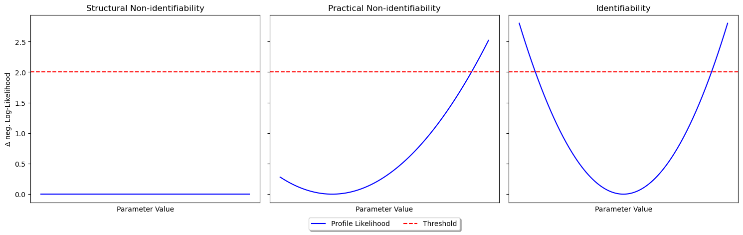
Generally, profile likelihoods can reveal the three different scenarios shown in the figure below.

• Structural non-identifiability of a parameter results in a flat likelihood profil.

• Practical non-identifiability, meaning the parameter is not identifiable given the data if the likelihood profile does not completely pass the confidence threshold.

• For a structural and practical identifiable parameter the profile likleihood exceeds the threshold in both directions.

The results of the profile_likelihood function can be shown using the plot_profile_likelihood function from the visualization submodule.

_ = visualization.plot_profile_likelihood(pl_result, estimates, show_coi=False)

5.6.2 Profile likelihood based Confidence Intervals

Given enough datapoints in the profile likelihoods, the results can be used to derive confidence intervals for the estimated parameters. The plot_profile_likelihood function can be called with show_coi=True to display likelihood based confidence intervals given a confidence level alpha.

_ = visualization.plot_profile_likelihood(pl_result, estimates,  alpha=0.05, show_coi=True)

Additionally, estim8 provides functions for calculating confidence intervals.

alpha = 0.05
threshold = calculate_negll_thresshold(alpha=alpha, df=len(estimates), mle_negll=est_info["fun"])

for parameter, pl in pl_result.items():
    par_values = pl[:,0]
    neglls = pl[:,1]
    coi = approximate_confidence_interval(par_values, neglls, threshold)
    print(f"{1-alpha} % Confidence interval for {parameter}: {coi}")

0.95 % Confidence interval for X0: (0.06913299729362944, 0.07915730866720107)
0.95 % Confidence interval for mu_max: (0.5283473082934588, 0.552359558967311)
0.95 % Confidence interval for Y_XS: (0.4830784248423862, 0.5129752888375013)