4 Modeling experimental replicates

This notebook demonstrates the replicate handling options provided by estim8. As a running example, the SimpleBatch model introduced in Notebook 1. Modeling & Simulation is used to create artificial data comprising to experimental replicates with varying conditions. It is shown how to model relations between experimental replicates using the ParameterMapping approach.

from estim8.models import FmuModel
from estim8.error_models import BaseErrorModel, LinearErrorModel
from estim8 import visualization, datatypes, Estimator, utils
import pandas as pd
import matplotlib.pyplot as plt

# load and init model
SimpleBatchModel = FmuModel(path=r'../../../tests/test_data/SimpleBatch.fmu')
# import datasheet
data = pd.read_excel(r'SimpleBatch_Data.xlsx', index_col=0, header=[0,1])
data.columns = data.columns.droplevel(1)
data

Time	X	S
0.0	0.176200	NaN
0.1	0.318313	NaN
0.2	0.285270	NaN
0.3	0.218600	NaN
0.4	0.248210	NaN
...	...	...
9.6	4.885956	NaN
9.7	4.807351	NaN
9.8	5.167874	NaN
9.9	5.220779	NaN
10.0	5.065959	0.0

101 rows × 2 columns

4.1 Parameter Mapping

In Estim8, model replicates are defined using a parameter mapping, which defines a hierarchy tree of global and replicate-specific “local” parameters.

# define replicate IDs
replicate_IDs = ['1st', '2nd']

# define an empty list for replicate specific parameters 
mappings = []

# define a different initial substrate concentration for the 1st replicate
mappings.append(utils.ModelHelpers.ParameterMapper(
    global_name='S0',            
    local_name='S0_1st',
    replicate_ID='1st',         
    value=15
    )
    )


# define replicate specific initial biomass concentrations
x0_vals = [
    0.11,   # 1st
    0.085   # 2nd
]

for rID, value in zip(replicate_IDs, x0_vals):
    mappings.append(
        utils.ModelHelpers.ParameterMapper(
            global_name='X0',
            local_name=f"X0_{rID}",
            replicate_ID=rID,
            value=value
        )
    )

parameter_mapping = utils.ModelHelpers.ParameterMapping(
    mappings = mappings,                                # the list of ParameterMappers
    replicate_IDs=replicate_IDs,                        
    default_parameters=SimpleBatchModel.parameters      # default model parameters
)

# display the mapping
parameter_mapping.mapping

		local name	value
global name	replicate ID
Ks	1st	Ks	0.010
	2nd	Ks	0.010
S0	1st	S0_1st	15.000
	2nd	S0	10.000
X0	1st	X0_1st	0.110
	2nd	X0_2nd	0.085
Y_XS	1st	Y_XS	0.350
	2nd	Y_XS	0.350
mu_max	1st	mu_max	0.400
	2nd	mu_max	0.400

The ParameterMapping object can be used to get the correct parameter set corresponding to a replicate_ID using its class method replicate_handling.

parameters_1st = parameter_mapping.replicate_handling('1st')
print(f'Parameters 1st: \n {parameters_1st}')

# run a simulation with parameters of 1st replicate
sim = SimpleBatchModel.simulate(0, 10, 0.1, parameters=parameters_1st)
_= visualization.plot_simulation(sim)

Parameters 1st: 
 {'Ks': 0.01, 'S0': 15, 'X0': 0.11, 'Y_XS': 0.35, 'mu_max': 0.4}

One can also pass a dictionary of parameters different to the default parameters of the ParameterMapping, but always refer to the local name of a parameter:

parameters_2nd = parameter_mapping.replicate_handling(
    replicate_ID='1st',
    parameters= {
        'S0': 1,          # will not be used, as it should be named as the local parameter "S0_1st" defined above
        'X0_1st': 0.15,   # correct reference to local parameter
        'mu_max': 0.4
        }
)
parameters_2nd

{'Ks': 0.01, 'S0': 15, 'X0': 0.15, 'Y_XS': 0.35, 'mu_max': 0.4}

4.2 Parameter estimation with replicates

4.2.1 Artificial noisy data

The SimpleBatch model introduced in Notebook 1 is used to create an artificial data set of two replicates based on the ParameterMapping defined above.

# define a function to create an artificial experiment
def make_experiment(parameters, model: FmuModel, original_data: pd.DataFrame, error_model: BaseErrorModel = LinearErrorModel(), rID: str = datatypes.Constants.SINGLE_ID, resample=4):
    simulation = model.simulate(t0=0, t_end=10, stepsize=0.1, parameters=parameters)

    measurements = []
    for obs in original_data.columns:
        model_prediction = simulation[obs]
        # get timepoints of measurements from datesheet above
        timepoints = original_data[obs].dropna().index
        values = model_prediction.interpolate(timepoints)
        # get noisy values by resampling the data according to erro models distribution
        for _ in range(resample):
            values = error_model.get_sampling(values=values,errors=error_model.generate_error_data(values), n_samples=1)[0]

        measurements.append(
            datatypes.Measurement(
                name = model_prediction.name,
                timepoints=timepoints,
                values=values,
                error_model=error_model,
                replicate_ID=rID
            )
        )
    return datatypes.Experiment(measurements, replicate_ID=rID)


# create noisy data
artificial_data = dict()
for r_ID in replicate_IDs:
    replicate_parameters = parameter_mapping.replicate_handling(
        replicate_ID=r_ID
    )

    artificial_data[r_ID] = make_experiment(parameters=replicate_parameters, original_data=data, model=SimpleBatchModel, error_model=LinearErrorModel(offset=0.05), rID=r_ID)

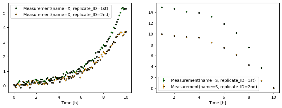
# plot data
fig, axes = plt.subplots(
    ncols=2,
    nrows=1,
    figsize=(12, 4)
)

for (r_ID, experiment), color in zip(artificial_data.items(), ['green', 'orange']):
    for ax, measurement in zip(axes, experiment.measurements):
        visualization.plot_measurement(ax=ax, measurement=measurement, color=color, ecolor=color)
        ax.set_xlabel('Time [h]')
        ax.legend()

Defining unknown parameters and their bounds is done analogously to the example above, where a dictionary of parameters was passed to the replicate_handling function by referring to a local name.

display(parameter_mapping.mapping)

bounds = {
    'X0_1st': [0.05, 0.2],
    'X0_2nd': [0.05, 0.2],
    'S0_1st': [1, 20],
    'mu_max': [0.2, 0.7]
}

		local name	value
global name	replicate ID
Ks	1st	Ks	0.010
	2nd	Ks	0.010
S0	1st	S0_1st	15.000
	2nd	S0	10.000
X0	1st	X0_1st	0.110
	2nd	X0_2nd	0.085
Y_XS	1st	Y_XS	0.350
	2nd	Y_XS	0.350
mu_max	1st	mu_max	0.400
	2nd	mu_max	0.400

4.2.2 Parallelized parameter estimation

# create an Estimator instance
estimator = Estimator(
    data=artificial_data,
    model=SimpleBatchModel,
    parameter_mapping=parameter_mapping,   # the parameter mapping 
    bounds=bounds,
    t = [0, 10, 0.1]            # t_start, t_end, stepsize_solver for simulation
)

# estimate
estimates, est_info = estimator.estimate(
    method='de',
    max_iter=1000,
    n_jobs=4,
)

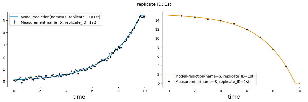
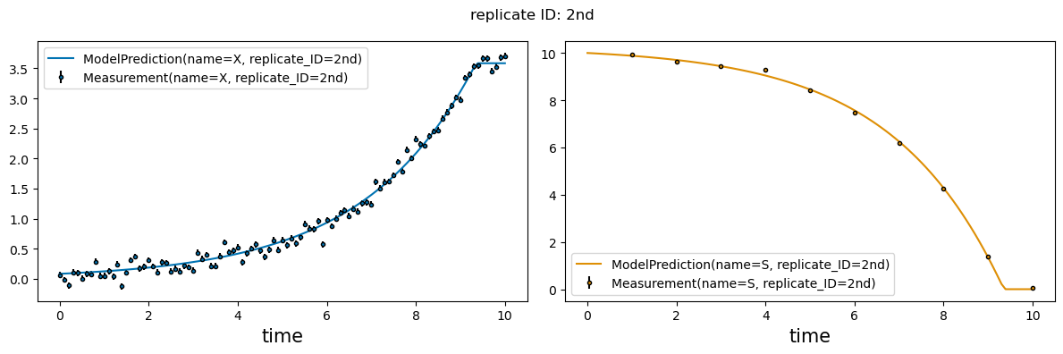
_ = visualization.plot_estimates(estimates=estimates, estimator=estimator, only_measured=True)

c:\Users\Latour\AppData\Local\miniforge3\envs\testim8\Lib\site-packages\scipy\optimize\_differentialevolution.py:487: UserWarning: differential_evolution: the 'workers' keyword has overridden updating='immediate' to updating='deferred'
  with DifferentialEvolutionSolver(func, bounds, args=args,